Introduction
In recent years, large language models (LLMs) have emerged as transformative tools in the field of natural language processing (NLP). These models, powered by deep learning, have achieved remarkable success in a wide range of NLP tasks, from text generation and translation to sentiment analysis and question-answering. The rise of LLMs, particularly transformer-based architectures, has revolutionized the way we approach language understanding and generation.
Transformers
At the heart of many LLMs lies the revolutionary transformer architecture. Transformers, as proposed in June 2017 in Attention Is All You Need, have reshaped the NLP landscape by replacing traditional recurrent neural networks (RNNs) and convolutional neural networks (CNNs) with a novel self-attention mechanism. This mechanism allows transformers to capture long-range dependencies in language, making them exceptionally effective at handling sequential data, like text.
Memory and Computational Challenges
While LLMs have unlocked new frontiers in NLP, they come with formidable memory and computational demands. These models are often vast in size, comprising millions or even billions of parameters. Such complexity offers remarkable linguistic capabilities but poses substantial challenges when it comes to running them on machines with limited resources.
In this study, we delve into the world of LLMs, transformers, and the intricacies of managing memory and computational constraints. We will explore the significance of addressing these challenges and the role of weight quantization, a memory optimization technique, in enabling the deployment of LLMs in resource-constrained environments.
Study Objectives
This research aims to achieve the following objectives:
- Understand the foundational concepts of large language models and transformers in NLP.
- Recognize the memory and computational challenges associated with running LLMs on machines with limited memory, such as Google Colab, which provides 12.7GB of RAM and 15GB of GPU.
- Introduce the concept of weight quantization as a means to reduce memory requirements.
- Implement and experiment with weight quantization techniques on pre-trained LLMs.
- Analyze the impact of weight quantization on memory usage, computational efficiency, and model performance.
Understanding Memory Constraints
Understanding memory constraints is crucial when working with LLM and other memory-intensive deep learning tasks.
Hardware Limitations of Google Colab
Google Colab is a popular cloud-based platform for running Python notebooks with access to free GPU resources. While it offers a convenient environment for deep learning experiments, it comes with memory constraints that can impact the execution of resource-intensive tasks. Google Colab provides:
- 12.7GB of CPU RAM
- 15GB of GPU RAM
Memory Constraints and LLM
LLMs, such as GPT-3 and other open-source models, are renowned for their immense parameter sizes, often exceeding hundreds of millions or even billions of parameters. These models require substantial computational resources, as we will understand later on, a 176 billion parameter model can require 352GB of GPU RAM to be ran! Consequently, loading and running such models in resource-constrained environments can pose significant challenges.
Introducing weight quantization
In this section, we delve into the concept of weight quantization, a memory optimization technique that plays a pivotal role in making LLMs feasible to run in resource-constrained environments. We will explore the fundamentals of weight quantization, its significance, and the two most common 8-bit quantization techniques: zero-point quantization and absolute maximum (absmax) quantization.
Common machine learning datatypes
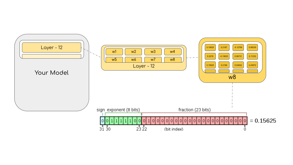
Before introducing Machine Learnigng (ML) datatypes, let’s do an recap. We are using transformers, which are a special type of contex-aware neural network. Like all neural networks, there are weights representing the importance of each of the neurons in network. Computers need a way to represent these weights (i.e. floating point numbers!).
Floating number representation
In the context of numerical representation, terms like precision (also mantissa or significand), range (also exponent) and sign come into play. Let’s break down each of these terms:
-
Sign Bit: is a single bit (binary digit) that determines the sign of the floating-point number, indicating whether it’s positive or negative. By using a sign bit, floating-point representation accommodates both positive and negative numbers within the same format. If the sign bit is 0, the number is positive; if it’s 1, the number is negative.
For example, In the number -42.0, the sign bit is 1 because it’s a negative number. In the number 3.14, the sign bit is 0 because it’s positive.
-
Range: controls the magnitude of the number being represented. It determines the scale or order of magnitude of the number. It allows the representation of both very large and very small numbers. It specifies how many positions the decimal point should be shifted to the left or right to express the actual value.
For example, in the number \(1.2345 × 10^3,\) “3” is the exponent. It indicates that the number should be scaled by \(10^3,\) which means it’s 1,234.5. The exponent controls the order of magnitude.
-
Precision: represents the fractional part of a floating-point number. It contains the significant digits that provide accuracy in representing a real number. It determines how finely you can represent values, especially those with many decimals. The more bits allocated to the precision, the greater the accuracy of the representation.
For example, in the number 1234.5678, the “1234” part is the integer portion, and the “5678” part is the precision or mantissa. It represents the fractional component with high accuracy.
Understanding these components is essential for dealing with numerical accuracy and precision in scientific and engineering computations.
We can also try this out on the web, follow this link and try to write your own decimal number into IEEE 754 format!
After this introduction on number representation we can start introducing some widely used ML dataypes:
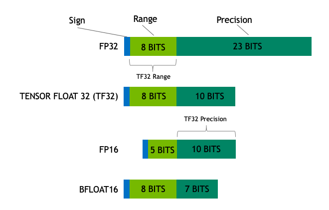
Float32 (FP32) stands for the standardized IEEE 32-bit floating point representation. With this data type it is possible to represent a wide range of floating numbers. In FP32, 8 bits are reserved for the “exponent”, 23 bits for the “mantissa” and 1 bit for the sign of the number. In addition to that, most of the hardware supports FP32 operations and instructions.
In the float16 (FP16) data type, 5 bits are reserved for the exponent and 10 bits are reserved for the mantissa. This makes the representable range of FP16 numbers much lower than FP32. This exposes FP16 numbers to the risk of overflowing, (trying to represent a number that is very large, too large for the range available) and underflowing (representing a number that is very small, too small for the range available).
A new format, bfloat16 (BF16), was created to avoid these constraints. In BF16, 8 bits are reserved for the exponent (which is the same as in FP32) and 7 bits are reserved for the fraction. This means that in BF16 we can retain the same dynamic range as FP32. But we lose 3 bits of precision with respect to FP16. Now there is absolutely no problem with huge numbers, but the precision is worse than FP16 here.
In the machine learning jargon FP32 is called full precision (4 bytes), while BF16 and FP16 are referred to as half-precision (2 bytes). On top of that, the int8 (INT8) data type consists of an 8-bit representation that can store \(2^8\) different values (between [0, 255] or [-128, 127] for signed integers).
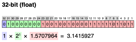
Practical example: π
Let’s to an exercise where we try to represent π using different datatypes. The first 71 digits of pi are 3.1415926535897932384626433832795028841971693993751058209749445923078164. However computers will have an hard time processing such a huge number. For our purposes we care about approximations of this number good enough that our model still perform as intended.
Using a float32 representation we will be:
While with a float16 we will have:
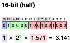
a very similar number hold for bfloat16, while for int8 π will be approximated to 3!
Datatype choice
While, ideally the training and inference should be done in FP32, it is two times slower than FP16/BF16 and therefore a mixed precision approach is used where the weights are held in FP32 as a precise “main weights” reference, while computation in a forward and backward pass are done for FP16/BF16 to enhance training speed. The FP16/BF16 gradients are then used to update the FP32 main weights.
During training, the main weights are always stored in FP32, but in practice, the half-precision weights often provide similar quality during inference as their FP32 counterpart – a precise reference of the model is only needed when it receives multiple gradient updates. This means we can use the half-precision weights and use half the GPUs to accomplish the same outcome.
To calculate the model size in bytes, one multiplies the number of parameters by the size of the chosen precision in bytes. For example, if we use the bfloat16 version of the BLOOM-176B model, we have 176*10**9 x 2 bytes = 352GB! As discussed earlier, this is quite a challenge to fit into a few GPUs.
But what if we can store those weights with less memory using a different data type? A methodology called quantization has been used widely in Deep Learning.
8-bit quantization
Experimentially, Huggingface has discovered that instead of using the 4-byte FP32 precision, we can get an almost identical inference outcome with 2-byte BF16/FP16 half-precision, which halves the model size. It’d be amazing to cut it further, but the inference quality outcome starts to drop dramatically at lower precision.
To remediate that, 8-bit quantization is introduced. This method uses a quarter precision, thus needing only 1/4th of the model size! But it’s not done by just dropping another half of the bits.
Quantization is done by essentially “rounding” from one data type to another.
For example, if one data type has the range [0,9] and another [0,4], then the value “4” in the first data type would be rounded to “2” in the second data type. However, if we have the value “5” in the first data type, it lies between 2 and 3 of the second data type, then we would usually round to “2”. This shows that both values “4” and “5” of the first data type have the same value “2” in the second data type. This highlights that quantization is a noisy process that can lead to information loss, a sort of lossy compression.
The two most common 8-bit quantization techniques are zero-point quantization and absolute maximum (absmax) quantization. Zero-point quantization and absmax quantization map the floating point values into more compact int8 (1 byte) values. First, these methods normalize the input by scaling it by a quantization constant.
For example, in zero-point quantization, if out range is [-1.0, 1.0] and we want to quantize into the range [-127, 127], we want to scale by the factor of 127 and then round it into the 8-bit precision. To retrieve the original value, we would need to divide the int8 value by that same quantization factor of 127. For example, the value 0.3 would be scaled to 0.3*127 = 38.1. Through rounding, we get the value of 38. If we reverse this, we get 38/127=0.2992 – we have a quantization error of 0.008 in this example. These seemingly tiny errors tend to accumulate and grow as they get propagated through the model’s layers and result in performance degradation.
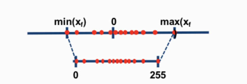
Now let’s look at the details of absmax quantization. To calculate the mapping between the fp16 number and its corresponding int8 number in absmax quantization, you have to first divide by the absolute maximum value of the tensor and then multiply by the total range of the data type.
For example, let’s assume you want to apply absmax quantization in a vector that contains \([1.2, -0.5, -4.3, 1.2, -3.1, 0.8, 2.4, 5.4]\). You extract the absolute maximum of it, which is 5.4in this case. Int8 has a range of [-127, 127], so we divide 127 by 5.4 and obtain 23.5 for the scaling factor. Therefore multiplying the original vector by it gives the quantized vector \([28, -12, -101, 28, -73, 19, 56, 127]\).
Discussion and analysis: loading Falcon 7B instruct
In this section we will (try to) load the model falcon-7B-instruct with weight quantised as float32, bfloat16, int8 and int4. Visit the Google Colab notebook here.
With float32: Memory Constraints
We will begin by attempting to load the Falcon 7B instruct model without any memory optimizations, using the standard float32 precision. This exercise aims to showcase the practical constraints posed by limited GPU memory.
from transformers import AutoTokenizer, AutoModelForCausalLM
import transformers
import torch

model = 'tiiuae/falcon-7b-instruct'

tokenizer = AutoTokenizer.from_pretrained(model)

pipeline = transformers.pipeline(
    "text-generation",
    model = 'tiiuae/falcon-7b-instruct',
    tokenizer=tokenizer,
    device = 'cuda',
    trust_remote_code=True
)
We are not able to load this model due to CPU crash. 12.7GB of CPU RAM are not enough even to load the architecture of a float32 quantised large laguage model with 7B parameters.
With bfloat16 quantised weights
The first quantisation technique we choose is the bfloat16, half-precision. This allows us to maintain the same range, so that we do not risk any underflow or overflow issues at the expense of some precision, i.e. decimals numbers.
from transformers import AutoTokenizer, AutoModelForCausalLM, TextStreamer
import transformers
import torch

model = 'tiiuae/falcon-7b-instruct'

tokenizer = AutoTokenizer.from_pretrained(model)

model_bfloat16 = AutoModelForCausalLM.from_pretrained(model,
                                                  device_map="auto",
                                                  torch_dtype=torch.bfloat16,
                                                  trust_remote_code=True)
During the model loading we observe peaks in the CPU RAM usage up to 12.5GB, which gets then unloaded and the model is transfered to the GPU RAM which gets 12.8 of its GB occupied.
After the model is loaded to the GPU we challenge it with the prompt “Tell me all about platypuses, common facts and also hidden gems”. It’s reply was
Platypuses are a unique species of egg-laying mammals found in Australia. They are known for their odd appearance, which includes a duck-like bill and a webbed tail. Some common facts about platypuses include that they lay eggs, have a bill that is shaped like a duck’s bill, and are found in the southern hemisphere. However, there are some hidden gems about these fascinating creatures. For example, did you know that they have venomous spurs on their hind legs? Additionally, they are the only species of monotreme that lay eggs.
In time: 104.944 seconds.
A bfloat16 uses 2bytes (16 bits) per parameter. Therfore \(7 \times 10^9 \times 2 = 14\times 10^9\) bytes, which are 14GB. This is consistent with the GPU usage for this model, which lays around 13GB. Discrepancies are due to approximations.
With int8 quantised weights
The second quantisation we approach is the int8, quarter precision!
from transformers import AutoTokenizer, AutoModelForCausalLM, TextStreamer
import transformers
import torch

model = 'tiiuae/falcon-7b-instruct'

tokenizer = AutoTokenizer.from_pretrained(model)

model_int8 = AutoModelForCausalLM.from_pretrained(model,
                                                  device_map="auto",
                                                  load_in_8bit=True,
                                                  trust_remote_code=True)
During model loading we observe CPU RAM utilization peaks aournd 12GB again and the GPU gets occupied for 8GB as we expected from theory:
$$ 7 \times 10^9 \times 1 = 7\times 10^9 \space bytes = 7GB $$
Notice that now multiply by one because the int8 datatype uses only 1 byte (8 bits) to represent a floating-point number! Discrepancies are due to approximations.
To the same question “Tell me all about platypuses, common facts and also hidden gems”, the model answered:
Platypuses are a unique species of egg-laying mammals found in Australia. They are known for their odd appearance, which includes a duck-like bill and webbed feet. Some common facts about platypuses include that they lay eggs, have a bill that is shaped like a duck’s bill, and are found in the southern hemisphere. However, some interesting facts about platypuses include that they are venomous, have a bill that is shaped like a duck’s bill, and are found in the southern hemisphere.
In time: 41.7087 seconds.
Altough an integer approximation could theoretically be a noisy process, we see that for this model and this prompt, the answer generated is quite consistent and similar to when weights are represented in half precision (bfloat16).
With int4 quantised weigths
An extra quantisation we have not talked about is int4. In theory it is as int8 but the representable range is lower.
import warnings
warnings.filterwarnings("ignore")
from transformers import AutoTokenizer, AutoModelForCausalLM, TextStreamer
import transformers
import torch

model = 'tiiuae/falcon-7b-instruct'

tokenizer = AutoTokenizer.from_pretrained(model)
streamer = TextStreamer(tokenizer, skip_prompt=True, skip_special_tokens=True)

model_int4 = AutoModelForCausalLM.from_pretrained(model,
                                                  device_map="auto",
                                                  load_in_4bit=True,
                                                  trust_remote_code=True)
GPU usage for this model sits around 5GB, as expected from theory. To the same prompt “Tell me all about platypuses, common facts and also hidden gems” the model replied
Platypuses are unique animals that lay eggs instead of giving birth to live young. They are found in Australia and New Guinea. Some common facts about platypuses include that they are venomous, have webbed feet, and lay eggs. Some hidden gems about platypuses include that they can swim, have a bill like a duck, and have a pouch on their chest where they lay their eggs.
In time: 55.956 seconds.
Summary
While all models have infered a decent answer, there are some things we can notice.
| bfloat16 | int8 | int4 |
|---|---|---|
| 13GB of GPU | 7GB of GPU | 5GB of GPU |
| Platypuses are a unique species of egg-laying mammals found in Australia. They are known for their odd appearance, which includes a duck-like bill and a webbed tail. Some common facts about platypuses include that they lay eggs, have a bill that is shaped like a duck’s bill, and are found in the southern hemisphere. However, there are some hidden gems about these fascinating creatures. For example, did you know that they have venomous spurs on their hind legs? Additionally, they are the only species of monotreme that lay eggs. | Platypuses are a unique species of egg-laying mammals found in Australia. They are known for their odd appearance, which includes a duck-like bill and webbed feet. Some common facts about platypuses include that they lay eggs, have a bill that is shaped like a duck’s bill, and are found in the southern hemisphere. However, some interesting facts about platypuses include that they are venomous, have a bill that is shaped like a duck’s bill, and are found in the southern hemisphere. | Platypuses are unique animals that lay eggs instead of giving birth to live young. They are found in Australia and New Guinea. Some common facts about platypuses include that they are venomous, have webbed feet, and lay eggs. Some hidden gems about platypuses include that they can swim, have a bill like a duck, and have a pouch on their chest where they lay their eggs. |
| 104.944 | 41.709 | 55.956 |
In bfloat16 we can observe that there is some repetition about the duck-like bill, but overall the result is statisfactory, also with a question asked back to the reader.
In in8 there is the same repetition present in the bfloat16 (repeated 3 times), and another one related to the southern emisphere. Also the detail about the venomomous spurs on the hind legs is just replaced with ‘they are venomous’.
In int4 the inference is shorted than the previous ones, but straight to the point without repetitions. Also it says about the pouch on the chest thatn in the int8 inference was not mentioned.
Overall we can observe a drastic cut in inference time using integer quantisation, at expense of some fluency. The model itself is not very big, for example the model working under the hood of chatGPT is called GPT-3.5-Turbo at its parameters are 175 trillion! Ours is 7 billion, 25000 times smaller! Altough at the time of writing, September 2023, some awarness regarding the fact that it is not only the number of parameters what matters but also the quality of data used for the model is made, at this small scale, a bigger model means better inference and as a consequence higher computational requirements.
Conclusion
In this study, we embarked on a journey to understand the challenges and solutions related to deploying LLMs, such as the Falcon 7B instruct model, in resource-constrained environments. We explored the significance of memory constraints, the role of different data types in representing model weights, and the impact of weight quantization techniques on model performance.
To address the computational resources demands of LLM, we introduced the concept of weight quantization, a memory optimization technique that allows us to reduce the memory requirements of LLMs.
We explored different data types, including float32, bfloat16, and int8, each with its trade-offs in terms of precision and memory efficiency. Through practical experiments, we observed that bfloat16 quantization can significantly reduce memory usage while maintaining model performance. Furthermore, int8 quantization, with its even smaller memory footprint, proved to be a viable option for inference tasks, albeit with a slight loss of precision.
In conclusion, memory constraints are a critical consideration when working with LLMs, and weight quantization techniques like bfloat16 and int8 provide effective strategies to make these models accessible in resource-constrained environments. The choice of quantization method should align with the specific requirements of the task, ensuring a balance between memory efficiency and model accuracy. As the field of NLP continues to advance, addressing memory and computational challenges will remain essential to democratizing access to cutting-edge language models.
Visit the notebook used for this study here.
References
https://huggingface.co/blog/hf-bitsandbytes-integration
https://huggingface.co/blog/accelerate-large-models
https://blogs.nvidia.com/blog/2023/01/26/what-are-large-language-models-used-for/
https://www.nvidia.com/en-us/glossary/data-science/large-language-models/
https://arxiv.org/abs/1706.03762
https://huggingface.co/learn/nlp-course/chapter1/4?fw=pt
https://huggingface.co/docs/transformers/perf_infer_gpu_one
https://evanw.github.io/float-toy/
https://colab.research.google.com/drive/1Gy3XSC7_fdQ9JS0bZiJuzsU7v81UqzZ2